In order to avoid unnecessary troubles and misunderstandings, it’s time for you to hide cells in Excel. MiniTool Partition Wizard introduces the steps to hide cells in Excel in this post. If you come across the same trouble, have a try.
Why Do You Need to Hide Cells?
Nowadays, the news about academic plagiarism and disclosure of trade secrets have aroused wide concerns in public. Hence, it is necessary to hide important data.
Besides, you may have been in some embarrassing situations. For instance, your colleague suddenly walks by when you are making the payroll forms of this month. Hiding what you do is a good choice for you.
Excel is one of the most common tools used to analyze data. If you want to keep the detailed data especially some information which causes great consequence, you could hide it. You can choose a part to hide such as a column, a row, or just a cell.
How to Hide Cells in Excel?
If you want to keep your files from being seen by your leaders, peers, or anyone has nothing with them, you can hide your cells in Excel. Just follow the following steps to have a shot at it.
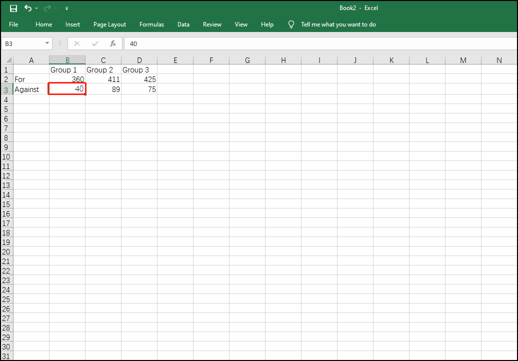
Step 1: After opening your file, the first step you need to do is to find the cell you want to hide. Now, taking the circled one for an example, you are supposed to right-click the cell.
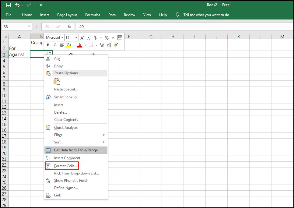
Step 2: Now, there is a popup window in front of you. You should scroll the mouse to Format Cells and hit it.
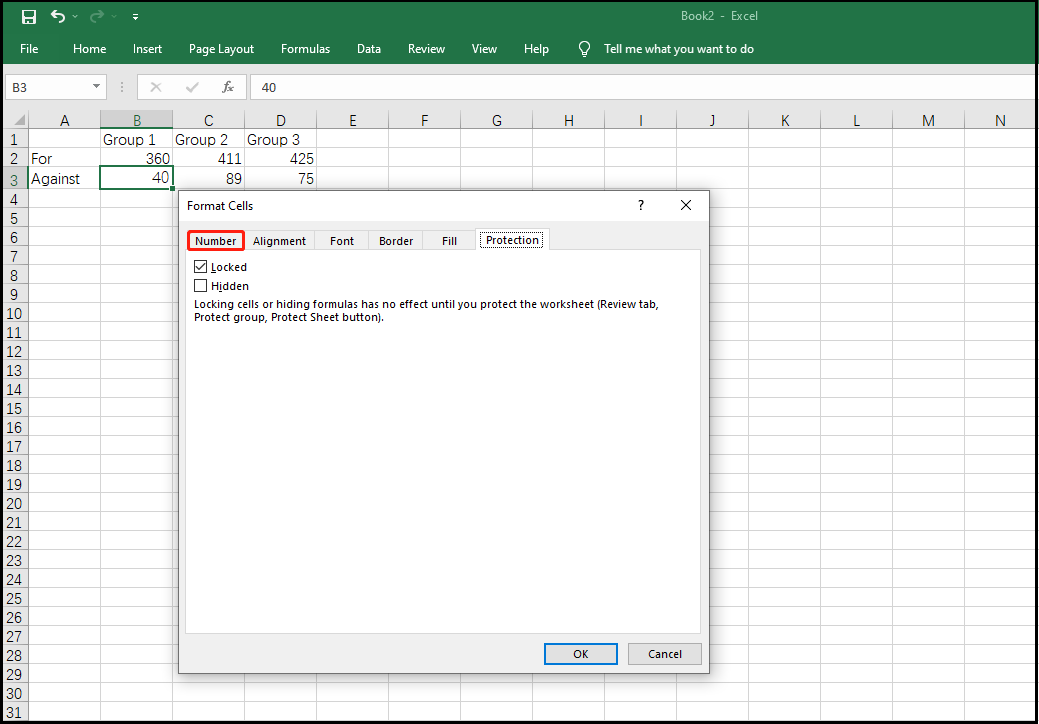
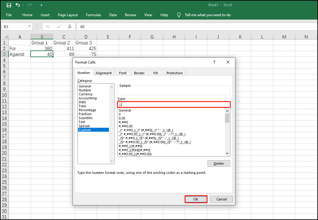
Step 3: A new interface appears. You ought to click Number.
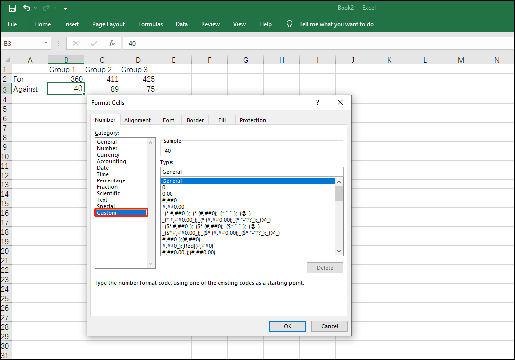
Step 4: In the selections of Number, you will see many options. Scroll down your mouse and choose Custom.
Step 5: Please pay attention to the changes of this interface. Find the blank in Type, and type “;;;” in this place. Then hit OK.
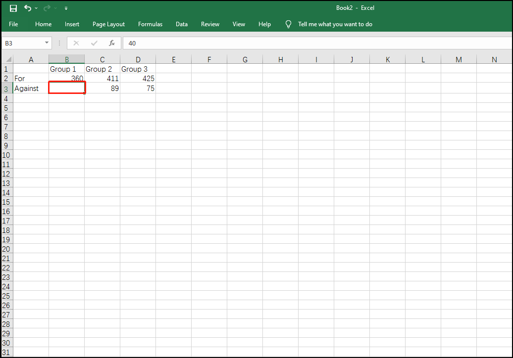
Step 6: Now, you have hided your target cell successfully. The next picture shows the result of your operations.
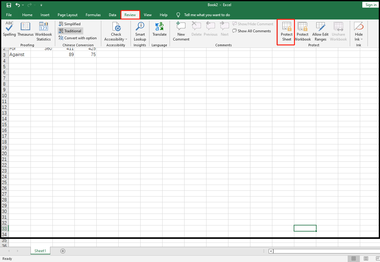
However, the steps above are not complete. As the user of Windows, you may know about Protect View. There are some procedures to protect cells in Excel you should follow.
Step 7: Please click the option of Review on the top of interface and select Protect Sheet.
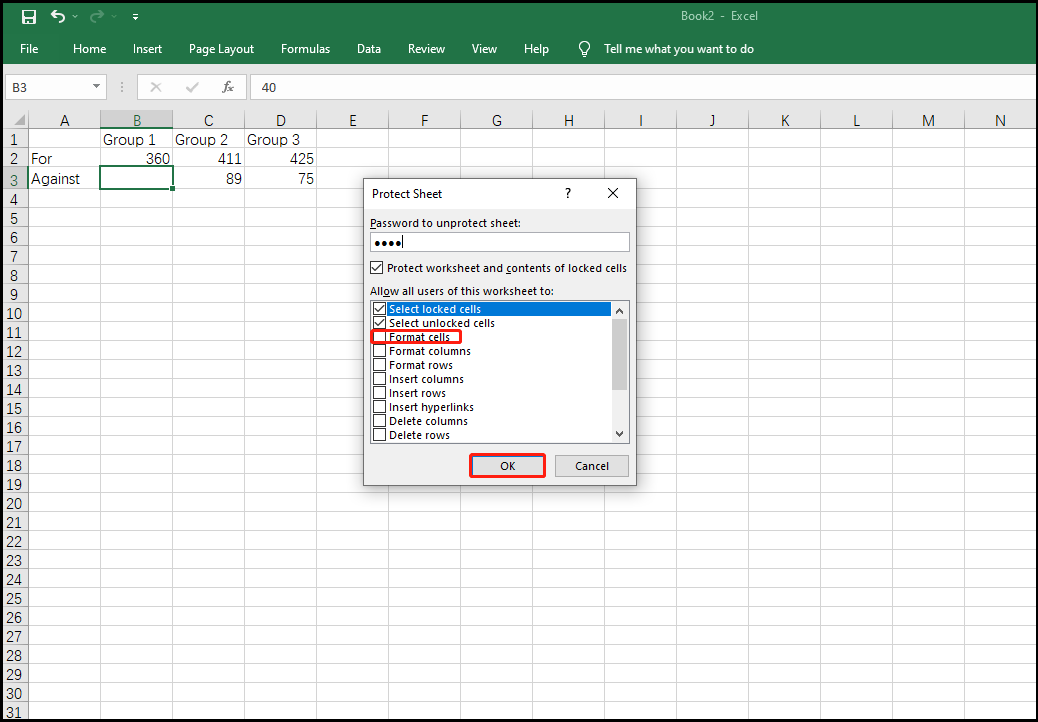
Step 8: After hitting Protect Sheet, there will be a new popup window. Look at the circled one under the Password to unprotect sheet, and input password.
Step 9: Look at this popup window again. Scroll your mouse to Allow all users of this worksheet to:, and then select Format cells and hit OK.
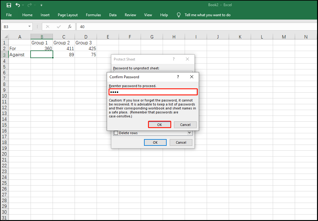
Step 10: There will be another popup window as shown below. Now, what you need to do is to reenter your reenter your password. Just input the password in the blank under Reenter password to proceed, and hit the option of OK.
Now, you have learned how to hide cells in Excel and how to protect cells in Excel. All the steps to hide your target cell in Excel have been described.
Read also: Excel Protected View: How to Remove It (Once and for All)?
Bottom Line
To sum up, this post has introduced the importance of hiding cells in Excel and the steps to hide cells in Excel. Hiding important files is an effective way to avoid information leakage and unnecessary misunderstanding. If you have encountered the same problem, you are supposed to follow the steps to solve. If you have any better ideas about it, you may share with us.
User Comments :