When you are using Excel to make a table, you can insert a check mark symbol to indicate “yes”. The check mark symbol is very useful, because the mark is more conspicuous and clearer than the text. This MiniTool post can help you add a check mark symbol in Excel easily.
Copy and Paste
This is the easiest way to insert a check mark symbol in Excel. You just need to right-click to copy ✓ here, and then you can simply paste this symbol into the Excel table. Of course, you can also press “Ctrl + C” to copy it, and press “Ctrl + V” to paste it.
Keyboard Shortcuts
If you want to directly enter a check mark symbol in Excel instead of copying the symbol from the web, you can use keyboard shortcuts.
- First, you need to change the font format to Wingdings.
- In the selected cell where you need to insert the check mark, press “Alt + 0252”.
In addition to the above shortcuts, you can also adjust the font format to Wingdings 2, and press “Shift + P” to add a check mark symbol in Excel.
Use Symbols Function
Besides, you can add a check mark with the symbol function in Excel.
- Select Insert from the ribbon above Excel.
- Then select the Symbols in the right area and then choose the Symbol dialog in the Symbols.
- In the Symbol dialog box, switch the font option to Wingdings, and then select the check mark symbol. Finally, click the Insert button.
Use AutoCorrect
You can use this AutoCorrect function to select a keyword, and when you enter the keyword, Excel will automatically turn it into a check mark. Of course, you can also use this method to replace the specified content in batches.
Follow the detailed steps below.
- Click on the File tab on the toolbar.
- Choose Options and then select Proofing from the Options dialogue box.
- Press the AutoCorrect Options button.
- In the AutoCorrect dialogue box, you can optionally enter a word in the Replace field, and paste checkmark character (✓) in the With field.
- Click the Add button to add this autocorrect rule. At last, click on OK to finish this operation.
You only need to add this auto-correction rule once, and you can continue to use this function in Excel later without repeating the operation.
Use the UNICHAR Formula
The methods mentioned above are only suitable for simple insertion situations, for example, you only want to insert a check mark in a few places. But it is not applicable if you need to insert a large number of check marks. In this case, it is best to use the formula to avoid the hassle of manual input.
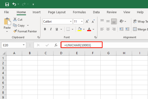
You can also directly use UNICHAR Formula in Excel to add check marks without changing the font.
Select the cell directly, and enter “=UNICHAR(10003)” in the place as shown in the picture below.
Use the CHAR Formula
This method is basically the same as the previous method, but with one more step. You need to format the font as Wingdings. Then, directly enter “= CHAR (252)” in the cell to insert a check mark.
In addition, combining the above two formulas with the IF formula can also help you insert a large number of check marks.
You can use the IF formula to specify that when the number exceeds a specific number, add a check mark after it, and even specify that when this requirement is not met, insert a cross mark (this mark can be obtained by entering “=CHAR(251)”) after it. The steps should be as follows:
- First, type your data in column A. Then, select a cell (eg. B1, which is after A1) in your Excel table and change the font to Wingdings.
- Type formula “=IF(A1>100,CHAR(252),CHAR(251))” in B1 and press Enter. You can apply this formula to the entire B column by pulling down B1.
The above formula means that if the number in the A column is more than 100, enter a tick mark (CHAR 252) in the corresponding B column. If not, enter a cross mark (CHAR 251) in the corresponding B column.
In conclusion, the above are six ways to add a check mark symbol in Excel, you can freely choose the one that suits you.
By the way, if you are suffering Microsoft Excel won’t open issue, you can try to resolve this issue by reading the following post.
User Comments :